Part One - Exploratory Data Analysis

Introduction #

The first step in any machine learning project, after defining the objective, is to explore the dataset. This is done to understand the nature of the data, as well as identify any feature correlations, redundancy, or other ways that we may be able to reduce the complexity of the dataset; leading to faster training, lower data storage requirements, and more accurate models.

With big thanks to the author, MaharshiPandya, this dataset was remarkably clean to begin with. There were 114,000 rows of data, split between 114 target classes (genres), each with exactly 1000 rows each.

Data Scaling #

Although none of the target classes had rows with missing data points, we did notice that the data did not maintain consistent scale across the numerical features. For example, the feature ‘popularity’ used a scale of 0 to 100, whereas ‘duration_ms’ was the length of the track in milliseconds, with a minimum of 8,586 and a maximum of 5,237,295. ‘Loudness’ had a minimum value of roughly -49 with a maximum of 4. This indicated that the data would require scaling prior to any model training. Additionally, there were several features that used numbers, but actually corresponded to categories. ‘time_signature’ had values ranging from 0 to 7, but referred to that value over 4 in reference to the time signature of a piece of music (ie: 3/4-time, 7/4-time, etc). It should be noted that 0/4 isn’t a valid time signature but did show up in the data and may simply refer to a piece of music that doesn’t have a set time signature or one that changes signature mid-song. ‘Mode’ is another feature that uses 0 or 1, but is a binary feature indicating whether a piece of music is in minor key. These categorical features would need to be dealt with prior to model creation and will be discussed in a later article in this series.

Correlating Features #

Feature correlation was the next area we examined, as highly correlated features ultimately add redundancy to the dataset. Removing redundant features reduces the size of a dataset, which not only can speed up the training process, but also means you don’t need to store the redundant data, leading to lower storage costs. Below is a correlation matrix for each feature. Each relationship is rated on a scale of 1 to -1, with the deeper red color (1) indicating that a feature is highly correlated, whereas the deep blue (-1) means the features are negatively correlated.

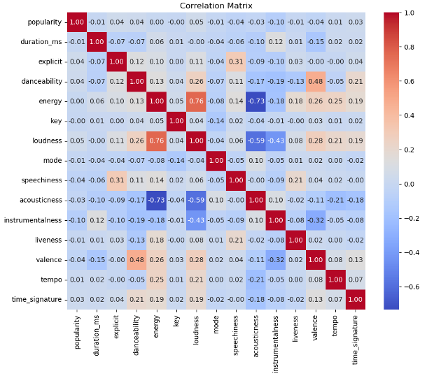
While there are several features with rather strong correlations, such as loudness and energy with a 0.76, acousticness and energy with a negative correlation of -0.73 and acousticness and loudness at -0.59, we ultimately decided to leave each of these features in the dataset. Later in this series of posts, we will perform some automated dimensionality reduction techniques, which may actually confirm whether we made the right choice of leaving these features in the dataset.

Wrap up #

This is the end of the Exploratory Data Analysis section of the project. In the next articles, I’ll cover the data preparation and pre-processing steps, where we remove several columns, scale the data, and make it ready for model training.